Monte Carlo SIL Calculations

Monte Carlo simulation is one of those things that everyone has heard of, but many people are not comfortable using it. One of the reasons people don’t use it is they think it requires fancy statistical tools. In todays post, I will be giving you a very brief introduction to using Monte Carlo simulation to incorporate uncertainty into your SIL calculations.

But wait, it gets better. I am not just explaining it. I will be demonstrating it and providing a free software tool for you to try it yourself. What is this fancy free software tool?

An Excel spreadsheet. 🙂

What is Monte Carlo?

Simply put, Monte Carlo (MC) simulation is a numerical technique that allows you to perform mathematical operations on random variables without “losing” the randomness in the result.

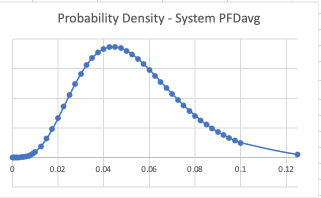
In the SIS world, our typical calculated output is PFDavg. This is determined using uncertain inputs such as the failure rate(s), proof test coverage, proof test interval, common cause, etc. Due to our uncertain knowledge (i.e. epistemic uncertainty), all of these input variables can be thought of as random variables and modeled via a probability distribution.

Monte Carlo simulation will repeatedly take random samples from the input distributions and calculate the output variable repeatedly based on whatever SIL equations we choose. The result of the MC simulation will be a probability distribution for PFDavg. As a result, the uncertainty in the input variables is propagated to the output variable.

For more on Monte Carlo, check out these more in depth tutorials here and here.

Software Tool

There are a lot of really useful commercial software tools out there for doing Monte Carlo simulation, including @Risk, ModelRisk, and Oracle Crystal Ball. They can do a lot of extra analysis that can be extremely valuable. However, if you just want to basic Monte Carlo, then Excel is all you need.

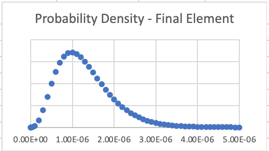
In the attached spreadsheet, we do a basic SIL calculation using simplified equations. Input variables are a failure rate, proof test interval, and proof test coverage for each of the sensor, logic solver, and final element. There is no redundancy, so we do not cover common cause. In addition, we have given a mission time for the system.

For illustration purposes, the simplified equation for each component is very basic:

PFDavg = Lambda*PTC*PTI/2 + Lambda*(1-PTC)*(Mission/2)

We define a distribution for each of our input variables. For more on estimating distributions, see this post and this paper. It is OK if the distribution is somewhat subjective based on your expertise and knowledge of the application.

The details of the MC simulation are better explained inside the spreadsheet and can be traced through the Excel formulas. So without further ado, here is the link to the tool:

Please comment below if you like the tool, or if you find any problems with it. Thanks for your support!