Bayesian Coin Flipping

The following is a quick example illustrating how the Bayesian updating process can be used to update prior knowledge based on new evidence. It is intended to be a fun and intuitive example. A similar approach can actually be used to analyze safety instrumented system (SIS) performance in the field.

Note: This quick example does not delve into details on e.g. how to choose a prior, the mathematical basis of Bayesian analysis, how to deal with non-homogenous data, etc. See further reading below for more information.

The Game

Let’s put forward two scenarios where you have an opportunity to play a coin flipping game. You have to pay $40 if you want to play the game. A coin will be flipped 100 times, and you get $1 for each time it comes up heads. Prior to playing, the coin will be flipped 10 times so you can judge if it is “fair”. The two scenarios are:

You have the opportunity to play with your sweet old grandma who just got a shiny brand-new quarter from the bank. Do you want to play?
Now you have a chance to play with One-Eyed Jack, who just got out of jail for counterfeiting and usually runs a game of 3-card monte behind the local liquor store. He has a crusty old coin from some country called Jackovia (wasn’t that in the Avengers movie?). Do you want to play?

A rational way to decide would be to use decision analysis and the expected values of the bets. How do we decide the expected value of a single coin flip? Is it always $0.50?

The Prior Knowledge

Obviously, our information on the two scenarios is uncertain and very different. We generally trust grandma, but what if she received a defective quarter? (why is there a heron on the back instead of an eagle? Seems fishy…) And what about that time she “forgot” to give you $5 for your birthday and went to play high-stakes Bingo instead? Hmmm.

One-Eyed Jack and his coin are obviously not to be trusted. He is a tricky fellow, but you did just see another guy win $5 off of him. The funky coin seems round, but is it really symmetrical? How to decide? We need more information!

But first, we need to quantify what we already know, as sketchy as that information may be. In this situation we will be subjective, although you could use information from a variety of sources to inform yourself, e.g.

Have an expert examine and measure both coins
Find some different quarters or Jackovia coins and flip them
Get feedback on One-Eyed Jack’s character from his known associates
Interview grandpa about grandma’s gambling habits

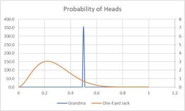
In the end, we decide that we strongly trust grandma and the U.S. mint, but we leave some possibility for defective coins, etc. The probability distribution for grandma’s coin is very narrow at 50% probability of heads.

For Jack, we suspect that he is scamming us, and the probability of heads is significantly less than 50%. We also think that if the coin always landed on tails you would have heard about it already. We are extremely confident that he would not be using a coin rigged in our favor! However, we are still very uncertain about the exact probability, so the distribution is wide and centered below 50%.

The two resulting subjective prior distributions are shown below:

We used Beta distributions for both grandma (a=100,000 B=100,000) and One-Eyed Jack (a=3 B=8).

The New Evidence

Armed with your prior knowledge, we proceed with the test flips:

Grandma flips it 10 times and comes up with 2 heads and 8 tails.
Jack flips it 10 times and it comes up with 5 heads and 5 tails.

OK, now that changes things! Or does it? Conventional statistics says that we have sampled the population and the mean is 20% for grandma and 50% for Jack, albeit with wide variance for both. However, that result does not pass the “funny look” test. Grandma might cry!

Instead, following our Bayesian approach, we can update the prior distribution with the new evidence. Since the Beta distribution is a conjugate prior for a Binomial likelihood, we can generate the posterior distribution just by adding our new data to the Beta distribution parameters (a,B) above:

Grandma: a’ = 100,000 + 2 = 100,002 B’ = 100,000 + 8 = 100,008
Jack: a’ = 3 + 5 = 8 B’ = 8 + 5 = 13

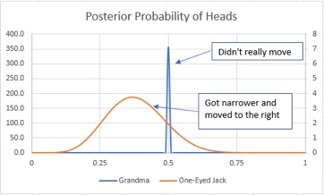
The resulting updated posterior distributions look like this:

We were already extremely confident in grandma, so the unusual results (2 heads, 8 tails) did not move the distribution. Our expected value from grandma moved from 50% all the way to 49.999%. Sweet old grandma would have to cheat us for years before we caught on!

The new evidence for Jack (5 heads, 5 tails) makes us feel a little better about Jack, but we still believe it’s likely he is trying to cheat us. However, the new evidence has moved the expected value from 27% to 38%. So, for a $40 dollar buy-in, we still should not play the game with Jack.

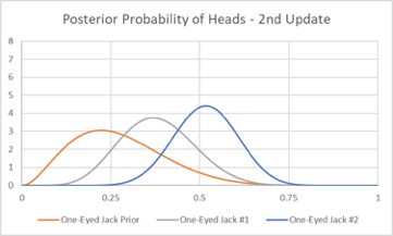
What if we told Jack we still were not sure and asked him to flip the coin 10 more times? If the new test resulted in 8 heads and 2 tails, we could simply repeat our updating process, and the new distribution would look like:

The new evidence causes the distribution to continue to narrow and move to the right. The new expected value is 52%, indicating that we should play the game with Jack, despite our earlier reservations. Game on!

A Common Objection

Some people might look at the above example and say “Oh noooo, that’s too subjective for me. I am an engineer! I deal with objective facts!”. However, these same folks probably have no problem picking a single point estimate for a failure rate based on data from TUV, exida, or OREDA. The reality is that failure rates and probability of failure on demand are uncertain. Building a distribution based on expert judgement (or other information) simply acknowledges and quantifies the uncertainty. Those who pick single point failure rate estimates are treating these data sources like grandma, i.e. so confident in the single value that it will never be updated regardless of later evidence.

On the other end of the spectrum from picking a single point estimate (similar to the “spikey” distribution for grandma) is prior use based on the traditional frequentist statistics approach, i.e. not considering prior knowledge. The frequentist approach is equivalent to using a flat / uniform prior distribution, indicating that all possible outcomes are equally likely. The Bayesian approach offers a middle ground between the spike and the flat distribution, allowing the initial estimate to be updated (and eventually dominated) by new data.

Wrap Up

Bayesian analysis allows us to incorporate prior knowledge, including both objective and subjective information into our analysis. It improves upon the implicit assumption of frequentist approaches that all outcomes are equally likely until proven otherwise by sampling. In situations where we truly “have no idea” about outcomes, Bayesian analysis can also use non-informative priors, which will give results very similar to frequentist approaches.

I hope this quick explanation was helpful without being too mathematical. I encourage you to read my paper “A Hierarchical Bayesian Approach to IEC 61511 Prior Use” to see an example of how to practically apply these concepts for failure rate data of Safety Instrumented Systems components.